Home Page | My Works | Seminar | BURP Thesis | Contents

CHAPTER SEVEN

Raster Data Model and Its Application

7.1 Introduction

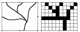
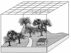
The raster data model is more like a photograph than a map. If a photograph is looked at through a strong magnifying glass, it will be seen that it is made up of a series of dots of different colors or shades of gray. The raster data model works in a similar way; it is a regular grid of dots (called cells, or pixels) filled with values. In fact, when a picture is stored in a computer, the raster data model is used.

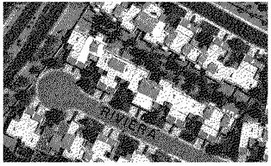In the photo below, there are streets, houses and vegetation. Notice that there are no boundaries drawn on the photograph to distinguish features; it is a continuous surface. Using the raster data model, the earth is treated as one continuous surface.

There are three ways to interpret each dot in the photograph. The first is to classify each dot as belonging to something - a group of similarly classified pixels becomes an object, like the street. The second way of interpreting is simply to measure the value of its color or shade of gray; the pixel on the upper left would be black, while the pixel on the bottom right would be medium gray. The third way is to define the pixel relative to a known reference point, such as mean sea level (for elevation) or the point of an oil spill. In the photograph above, the height of buildings and vegetation could be measured relative to street level.

The same three interpretations can be used for the raster data model in GIS. The cell value can represent a classification, such as vegetation type. It can be a measurement, such as a satellite measuring the amount of light reflected by the earth. Finally, it can be an interpretation of elevation (ESRI, 1998).

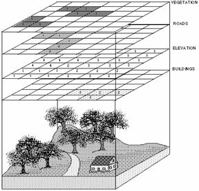
7.2 Structure of Raster Data Model

In the raster data model, each location is represented as a cell. The matrix of cells, organized into rows and columns, is called a grid. Each row contains a group of cells with values representing a geographic phenomenon. Cell values are numbers, which represent nominal data such as land use classes, measures of light intensity or relative measures.

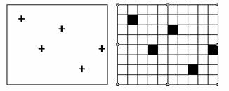
Like the vector data model, the raster data model can represent discrete point, line and area features. A point feature is represented as a value in a single cell; a linear feature as a series of connected cells that portray length; an area feature as a group of connected cells portraying shape (as above).

The accuracy of a map depends on the scale of the map. In the raster model, the resolution, and hence accuracy, depend on the real-world area represented by each grid cell. The larger the area represented, the lower the resolution of the data. The smaller the area covered, the greater the resolution and the more accurately features are represented.

Because the raster data model is a regular grid, spatial relationships are implicit. Therefore, explicitly storing spatial relationships is not required as it is for the vector data model.

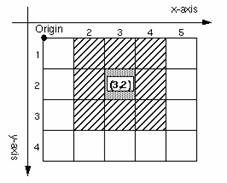
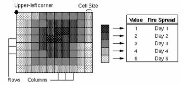
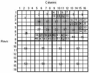
Notice that in a grid, cells have eight (8) neighbors (except those on the outside edges); four off the corners and four off the sides. Cells are identified by their position in the grid. In the example beside, with an origin in the upper-left, the cell (3, 2) would be 3 over along the x-axis and 2 down on the y-axis. Finding any one of eight neighbors simply requires adding or subtracting one (1) from the x or y values. For example, the value to the left of (3, 2) is (3-1, 2) or (2, 2).

Raster data is georeferenced by specifying the coordinate system to which a grid is registered, the real-world location of the reference point and the cell size in real-world distances. Typically, the upper-left or the lower-left corner of the grid is used as the reference point. This reference point location, along with the cell size, can be used to determine the geographic location of any cell within the raster data set. Using the same coordinate system, raster data sets can be logically organized into subjects for geographic analysis (ESRI, 1998).

7.3 Methods for Determining Raster Cell Values

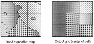
There are four main methods for determining cell values:  centroid, predominant type, most important type and percentage breakdown. Each method has been designed to represent a certain type of data better than the other. The choice of method depends on the type of data to be gridded and the analysis to be performed. GRID currently supports the predominant type and most important type of gridding methods.

Centroid method

Using this method, each cell is assigned the value of the feature that passes through the center of the cell. This method can be used for any feature type, but is particularly useful in coding continuous data, such as elevation, noise movement, or fluid flow. It will be at that location (the center of the cell) that a sample will be taken and a surface value will be recorded (ESRI, 1998).

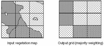
Predominant type method (majority weighting) 

The value of the feature that fills the majority of the cell is assigned to the location. Consider, for example, that a grid is overlaid in the gridding process onto a vegetation coverage. A particular cell resulting from the process consists of 20 percent oak, 35 percent maple, and 45 percent pine. With the predominant-type gridding, the cell will receive the value associated with the pine feature class since pine fills more of the cell than any other vegetation type. This method is good for discrete or noncontinuous data such as land cover, vegetation, or soils, where the boundaries of the objects can be defined and their associated value assigned to the cell when it occupies the majority of the cell (ESRI, 1998).

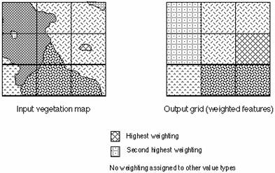
Most important type method 

Each cell is assigned the value associated with the features that have been specified as more important to the study. For example, if someone is studying the vegetation of a particular area, he may want to retain the identity of locations or zones that contain endangered plant species, even if the endangered plants don’t fill the majority of the grid cell or fall at the center of the cell (ESRI, 1998).

Percentage breakdown method

In this method, a cell is assigned several values, one per feature, according to the percent each feature occupies within the cell. This is a difficult and costly method to implement at data entry. However, it can be especially useful for statistical data (ESRI, 1998).

7.4 Raster Storage and Compression Techniques

Compression techniques have been developed to reduce the size of a cell-based database. Data consisting of large homogeneous features can be compressed better than data consisting of small fragmented polygons. Specific compression techniques compress some data better than others, but no compression technique compresses all types of data more effectively than another. The popular compression techniques are discussed bellow (ESRI, 1998).

Cell-by-cell 

For data that has a unique value for every cell, there is no way to compress the information. This is usually true for floating-point grids or continuous surfaces such as elevation data, slope surface and noise pollution grids. The row and column identify the location, and the value defines the attribute.

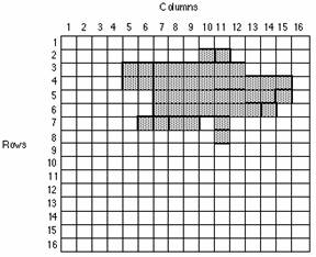
Cell-by-cell storage of the simple grid above may appear as follows,

1,1 : 0;1,2 : 0; 1,3 : 0, ....1,16 : 0

2,1 : 0;2,2 : 0; ...2,10: 1, 2,11 : 1; ... 2, 16 : 0

3,1 : 0;3,2 : 0; ... 3,5 : 1;3,6 : 1;3,7 : 1,3,8 : 1 ....

…

…

The first value represents the row number and is followed by a comma. The second value is the column number. The number after the colon is the value assigned to the cell. The actual storage of the cell-by-cell code in the computer may vary widely according to the implementation of the theory by the software.

Run-length code

When adjacent cells have the same value, runs are created and the data can be compressed. Run-length coding stores data by row. A row is identified first, followed by the columns and the value associated with the row-column location. The column range information is stored as a from-column to a to-column along with the value that is associated with that cell or group of cells. If two or more adjacent cells have the same value, only the from- and to-columns and the value are stored. The more columns that can be included in the from- and to-column identification as having the same value, the greater the compression will be.

To represent the above grid in run-length code may look as follows,

1 : 1 - 16 : 0

2 : 1 - 9 : 0; 10 - 11 : 1; 12 - 16 : 0

3 : 1 - 4 : 0; 5 - 12 : 1; 13 - 16 : 0. . .

Quad tree

The quad-tree approach for coding first divides a grid (or matrix) into four equal, smaller squares when cells in the grid have different values. If all the cells within any of the four smaller squares have the same value, the square will not be broken down any further. However, if there are cells with different values, (therefore the square does not consist of all homogenous cells), that square has to be subdivided into four more equal squares. This process continues until each square only represents cells with the same values.

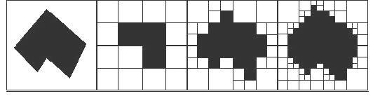
The quad tree is so named because the squares are stored in a hierarchical tree. The tree starts with one branch and then produces four branches. Each time a square is divided, it is always divided into four more branches, and the quad tree grows a level. When the quads or squares no longer need to be subdivided, a value is assigned to represent each branch and level.

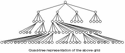
As with all compression techniques, information of the processing cell’s immediate 3 x 3 neighborhood or its extended neighborhood is not stored with the cell. To obtain information on the neighboring cells and their values as they relate to a single cell, the grid must be expanded to the original row-column grid. Depending on the data and the compression technique, this may be costly, thus slowing all processes and analyses that require this expansion.

7.5 Special Type of Raster Data Model

DEM (Digital Elevation Model)

A Digital Elevation Model (DEM) is an ordered array of numbers that represents the spatial distribution of elevations above some arbitrary datums in the landscape (Moore, 1993). In principle, a DEM describes the elevation of any point in a given area in digital format and contains information of the so-called ‘skeleton’ lines. Skeleton lines are lines of slope reversals (drainage, crests) and breaks of slope.

 A Digital Terrain Model (DTM) includes the spatial distribution of terrain attributes. A DTM is a topographic map in digital format, consisting not only of a DEM, but also the types of land use, settlements, types of drainage lines and so on.

Morphometric terrain units are mapping units, which group characteristics of the terrain. These include internal relief, form of the drainage divides (convex, flat, sharp, etc), slope from (straight, convex, concave, irregular, etc.), the drainage density and type of patterns and other characteristics of the drainage network within the units (Speight, 1977, Meijerink , 1992). The boundaries of these polygons, with the associated attribute values, can be stored digitally, but the units do not constitute a model suitable for manipulation.

Although generally associated with the land surface, a DEM may also describe a groundwater surface or the configuration of the bottom of an aquifer.

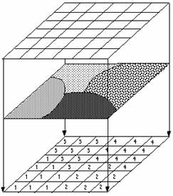
GRID

Grid-based systems, like vector-based systems, store geographic data, but they view and store surfaces differently. Vector systems define an object and proceed to define its characteristics and attributes. One of these characteristics is the x, y coordinate location. Grid-based systems divide the world into discrete uniform units called cells. Every cell represents a certain specified portion of the earth, such as a square kilometer, hectare or square meter. Each cell is given a value to correspond to the feature or characteristic that is located at or describes the site, such as a drainage basin, soil type, or residential classification. Location is not defined as an attribute but is inherent in the storage structure.

The uniform cells are organized into a Cartesian matrix consisting of rows and columns. A row identifies all cells equidistant from the top or bottom boundary of a grid. Columns identify all cells equidistant from the left or right boundary of the grid. Each Cartesian matrix is called a grid. Every cell in a grid has a unique row and column identifier.

The gridding process is like draping a fishnet containing square cells over the study area. A code is assigned to each cell (depending on the coding technique chosen) according to the feature that either is at the center of, fills the majority of, or is a special feature that is contained in the cell. The code or value of a cell is a numeric value that corresponds to an attribute type. Numeric values speed processing and allow for data compression.

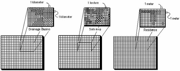
Each cell represents a specified portion of the world. A cell can be any size defined; there are usually no practical limits. The main consideration is that the size be appropriate for the analysis. For example, normally a 1-kilometer cell size should not be used when studying field mouse habitat.

This gridding procedure is the same when deriving a grid from an existing map. The values assigned to the cell correspond to a polygon attribute (or whatever item the polygon is gridded on) and create a representation of the real world.

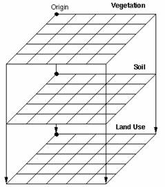
In most grid-cell databases, data about a particular site is divided into homogeneous features or classes and mapped as separate layers. Each layer contains all the features that fall into a similar classification, or are logically grouped together for future analysis. A grouping is a set of items, features, or characteristics that share a relative logic. These layers conform to feature or theme maps, and there is one grid for each layer. There is usually one feature or theme per grid (ESRI, 1998).

7.6 Application of Raster Data Model

Air pollution intensity mapping of Khulna City as Health Risk to Urbanite

Air pollution is a major environmental health problem affecting developed and developing countries around the world. Increasing amounts of potentially harmful gases and particles are being emitted into the atmosphere on a global scale, resulting in damage to human health and the environment. It is damaging the resources needed for the long-term sustainable development of the planet (WHO, 1999).

There is no doubt that air pollution is generally detrimental to health, especially to the respiratory system.  Air pollution may not only cause the abrupt onset of symptoms, producing severe ill-effects and sometimes even death (acute effects), but it might also have longer-term chronic effects (ERMP, 2001). Comparative Environmental Risk Assessment (CERA, 1998) for Khulna city depicted, presence of higher level of SO_x, NO_x and SPM in the ambient air of Khulna city; particularly in the city’s industrial areas, bus stations and commercial areas. In this study an air pollution intensity map is prepared considering the concentration of SOx, NOx and SPM in ambient air based on WHO health based standard. This study shows the application of raster data model and the capability of raster GIS.

7.6.1 Rationale

The world has witnessed an impressive growth in the economy and in industrialization during this century. Industrial growth in the world has been accompanied with worsening air quality in its cities. Given the spatial nature of air pollution, creating a map of the extent and concentration of air pollution would be an obvious thing to do (Briggs et al. 1997). Air pollution causes much harm to human life in many cities of the world. Dhaka, the capital city of Bangladesh has already been dangerously polluted. The effect of air pollution is clear to everybody today. So there should be a data to know the intensity of pollutant and air quality of every spot of Khulna City.

7.6.2 Type of air pollutant

Air pollutants are usually classified into suspended particulate matter (dusts, fumes, mists, and smokes), gaseous pollutants (gases and vapors) and odors.

Suspended particulate matter (SPM) Particulate matter suspended in air includes total suspended particles (TSP), PM₁₀, (SPM with median aerodynamic diameter less than 10 µm), PM_2.5 (SPM with median aerodynamic diameter less than 2.5 µm), fine and ultrafine particles, diesel exhaust, coal fly-ash, mineral dusts (e.g. coal, asbestos, limestone, cement), metal dusts and fumes (e.g. zinc, copper, iron, lead), acid mists (e.g. sulphuric acid), fluoride particles, paint pigments, pesticide mists, carbon black, oil smoke and many others. Suspended particulate pollutants provoke respiratory diseases, and can cause cancers, corrosion, destruction to plant life, etc. They can also constitute a nuisance (e.g. accumulation of dirt), interfere with sunlight (e.g. light scattering from smog and haze) and also act as catalytic surfaces for reaction of adsorbed chemicals (WHO, 1999).

Gaseous pollutants: Gaseous pollutants include sulphur compounds (e.g. sulphur dioxide (SO₂) and sulphur trioxide (SO₃)), carbon monoxide (CO), nitrogen compounds [e.g. nitric oxide (NO), nitrogen dioxide (NO₂), ammonia (NH₃)], organic compounds [e.g. hydrocarbons (HC), volatile organic compounds (VOC), polycyclic aromatic hydrocarbons (PAH) and halogen derivatives, aldehydes, etc.], halogen compounds (HF and HCl) and odorous substances (WHO, 1999).

Secondary pollutants may be formed by thermal, chemical or photochemical reactions. For example, by thermal action SO₂ can be oxidised to SO₃ which, dissolved in water, gives rise to the formation of sulphuric acid mist (catalysed by manganese and iron oxides). Photochemical reactions between NO_x and reactive hydrocarbons can produce ozone (O₃), formaldehyde (HCHO) and peroxyacetyl nitrate (PAN); reactions between HCl and HCHO can form bis-chloromethyl ether.

Odors: While some odors are known to be caused by specific chemical agents such as hydrogen sulphide (H₂S), carbon disulphide (CS₂) and mercaptans (R-SH, R₁ S R₂), others are difficult to define chemically (WHO, 1999).

7.6.3 Working Process

The intensity of pollutant at 13 point of Khulna City has been distributed to the cell of DEM through interpolation of the 3 major pollutant data.

Point interpolation (ANNEXURE C) has been used to generate DEM in this study. Volume of pollutant at the sample point has been interpolated through IDW (Inverse Weighted Distance) method as it can distribute data smoothly to the surface of DEM unlike methods like Spline, Kriging and Trend. The parameters of the analysis at ArcView Spatial Analyst was –

Output Grid Cell Size: 5m (a pixel represent 5m of real area)

Method: IDW

Z Value Field: Pollutant Volume data (as this data have to be distributed to the DEM)

Nearest Neighborhood (to let the interpolation be irregular according to points)

Number of Neighbor: 6 (to minimize the influence of far point)

Power: 2 (distance between points will be squared in interpolation process which will control the surface smoothness)

Barriers: No Barriers 

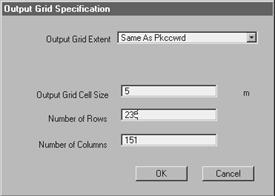
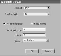
Figure 7.1: Parameters of Interpolation

Grouping of the pollutant

The interpolated DEM has been grouped using WHO’s (World Health Organization) health based standards NOx 100 mg/m³, Sox 80 mg/m³, SPM 150 mg/m³ (WHO, 1999) the groupings are presented in Table 7.1.

Table 7.1: Grouping of the pollutant according to WHO health based standard

Reclassification can produce a new map of the same geographical area with new cell value of DEM. The three DEM has been reclassed according to table 2.1. Example: the cell value range 0 to 50 will be reclassed as 1, cell value range 50 to 100 will be reclassed as 2 in case of NOx and so on. Through weighted overlay of three pollutants DEMs, comparative air quality map of Khulna City has been prepared in ArcView Model Builder. The Model is shown in Figure 7.2.

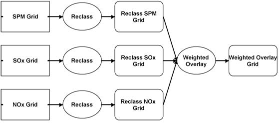
Figure 7.2: Model for Weighted Overlay of three DEMs

The parameters of model builder

The parameter used to reclass the interpolated grid theme to prepare input of weighted overlay is presented in Table 7.2.

Table 7.2: Parameters of reclassification

The cell size of the reclassed grid has taken 5 m and the analysis extent of the model has taken the polygon of the area of Khulna City that is the boundary of Khulna City.

In weighted overlay the reclassed grid theme has been used as input data. The evaluation scale has set 1 to 5 to keep the result with in 5 groups. The influence level of the theme was 35% for SOx, 35% for NOx and 30% for SPM accordingly their toxicity to human health.

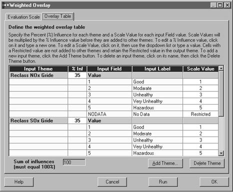
Figure 7.3: Parameters of Weighted overlay

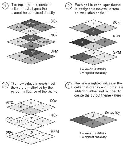
Figure 7.4: Example of Weighted Overlay process

The output interpolation is a rectangular area which contains area within and outside Khulna City. To calculate the area coverage of pollutants within Khulna City the raster has been clipped by Khulna City boundary with an Avenue Script (ANNEXURE B). Then the reclassed DEM has been converted to vector Shape file. The area in acre has been calculated using another Avenue Script (ANNEXURE B).

7.6.4 Findings

1. Pollution caused by NOx in Khulna City

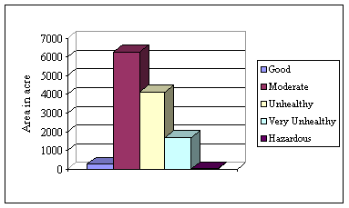
All the five groups of NOx level are present in Khulna City. Map 7.1 shows the air pollution caused by NOx in Khulna City. Total area coverage of moderate air condition considering NOx is high in Khulna City which is 6258.617 acre. Area coverage of unhealthy and very unhealthy air quality is 2^nd and 3^rd respectively. Table 7.3 and Figure 7.5 show the situation.

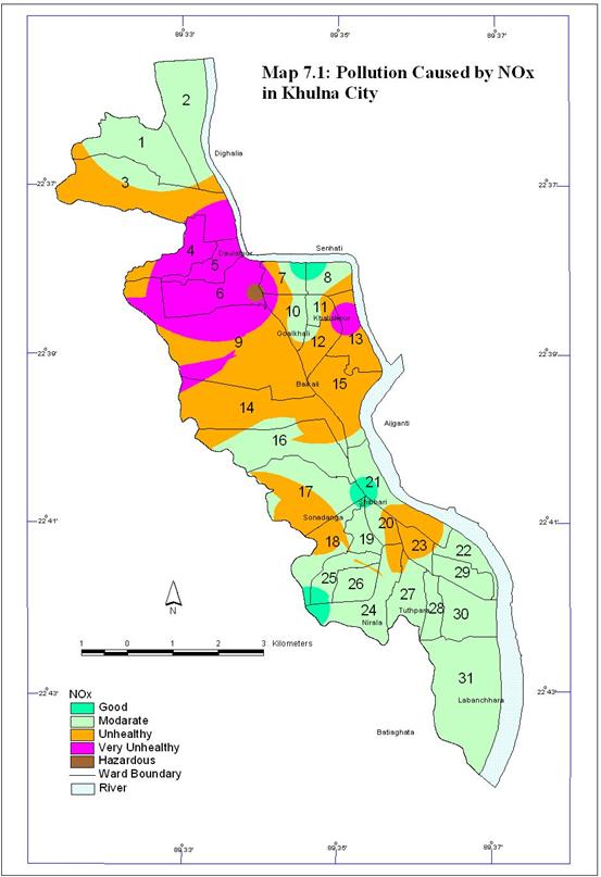
Table 7.3:  Area coverage of NOx in Khulna City

Figure 7.5: Area coverage of NOx in Khulna City

2. Pollution caused by SOx in Khulna City

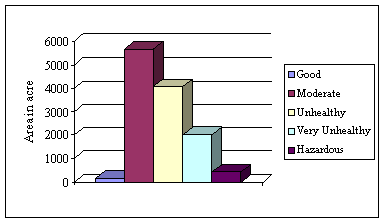
SOx pollutant is found in Khulna City at a dangerous level. More than half area of Khulna city lies above normal level. Map 7.2 shows air pollution caused by SOx in Khulna City. Good air condition considering SOx is very low and a large area is covered by moderate quality air. Area coverage of SOx is shown in Table 7.4 and Figure 7.6.

Table 7.4: Area coverage of SOx in Khulna City

Figure 7.6: Area coverage of SOx in Khulna City

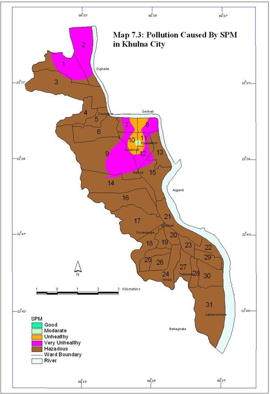
3. Pollution caused by SPM in Khulna City

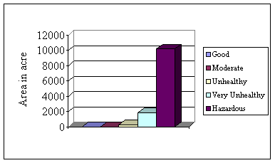
Concentration of SPM is very high in the air of Khulna City. Map 7.3 shows the concentration of SPM in the air of Khulna City. There is no place where the air quality is good considering the level of SPM. The area coverage gradually increases from moderate to hazardous air quality. SPM concentration of hazardous level is present at a large area in Khulna City. The area coverage of SPM concentration according to level is shown in Table 7.5 and Figure 7.7.

Table 7.5: Area coverage of SPM in Khulna City

Figure 7.7: Area coverage of SPM in Khulna City

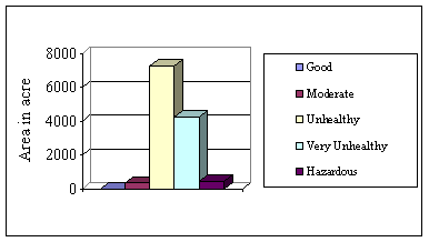
4. Comparative air quality of Khulna City

To be a healthy air all the pollutants have to be at normal level. But presence of only one pollutant at above normal level will be risky for health. With this concept most of the place of Khulna City is risky. In this study integrating the value of three major pollutants, the comparative air quality of Khulna City has been prepared. The integrated air pollutant concentration of Khulna City is presented in Table 7.6 and Figure 7.8. The result shows that there is no place where Comparative air quality is good. In weighted overlay every individual layer has influence to the output. So as there is no place good considering SPM, integrated DEM has no good air condition at any place of Khulna City. Moderate air condition prevails only in 370.164 acre area. 4 acre area of Khulna City is above normal quality. Pollutant concentration of 12006.754 acre area of Khulna City is above normal. Map 7.4 shows the comparative air pollutant concentration of Khulna City.

Table 7.6: Area coverage of air pollutant in Khulna City (comparative level)

Figure 7.8: Area coverage of air pollutants (comparative level)

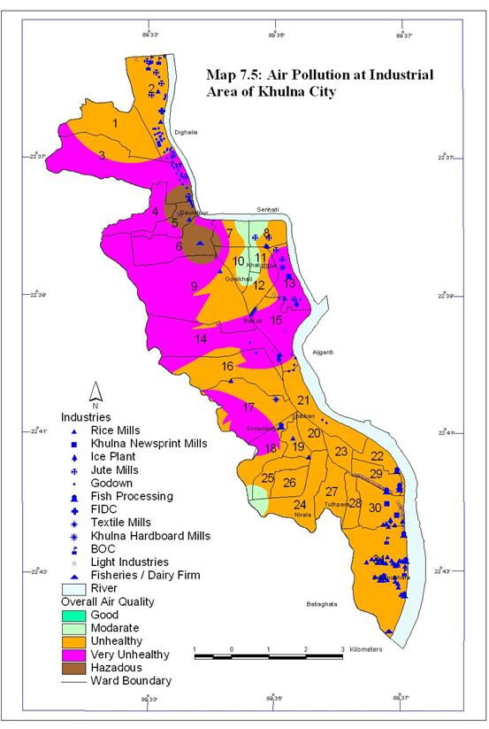
The pollutants considered here are generally emitted from industries and motor vehicles. All types of industry do not emit all pollutant but they have at least some contribution to the pollutant emission. The air pollution DEM with respect to the industries of Khulna City is presented in Map 7.5.

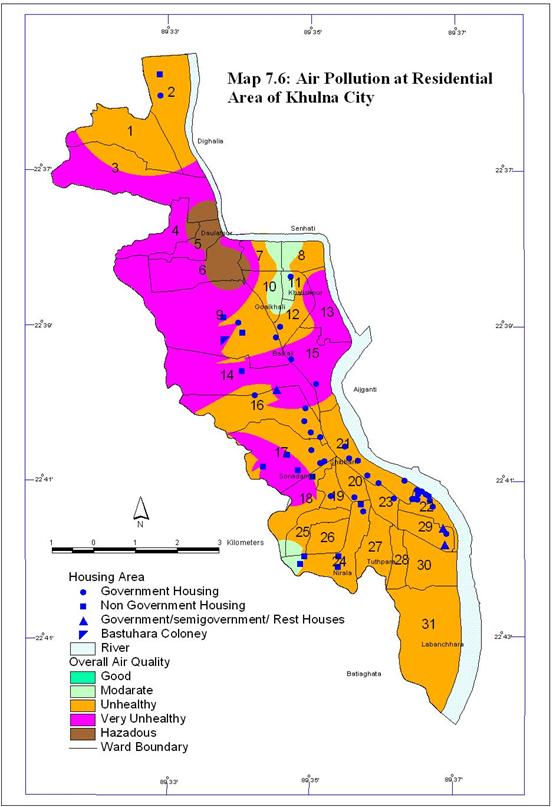
Map 7.6 shows the condition of air of the residential areas of Khulna City. The study finds that the air quality of many residential areas of Khulna City is unhealthy according to WHO standard.

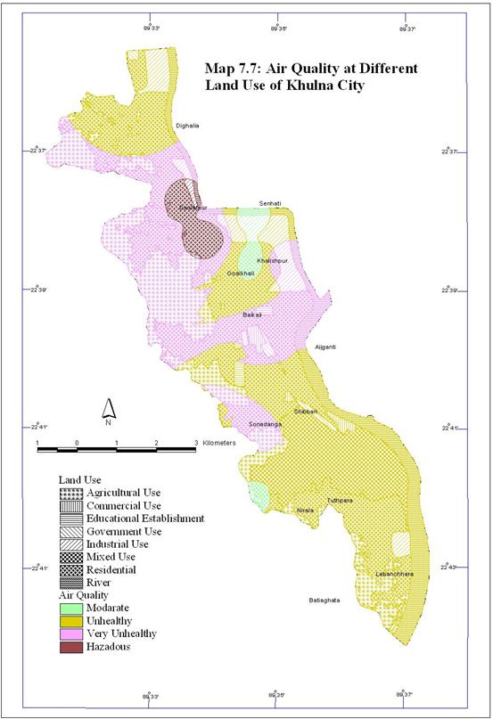
Land use also has significant influence on air pollution in a city.  Different land use causes air pollution differently and also different land use become victim of air pollution differently that is air pollution tolerance level is different in different land use. In fact there is no such pattern of air pollution with land use in Khulna City. The integrated air quality with land use is shown in Map 7.7.