Home Page | My Works | Seminar | BURP Thesis | Contents
CHAPTER FIVE
Data Model
The human eye is highly efficient at recognizing shapes and forms, but computer need to be instructed exactly how spatial patterns should be handled and displayed (Burrough, 1993). Geographical variations in the real world is infinitely complex the closure it can be looked the more detail can be seen almost without any limit. It would take an infinitely large database to capture the real world precisely. So data must be somehow reduced to a finite and manageable quantity by a process of generalization or abstraction. Geographical variation must be represented in terms of discrete elements or objects (Goodchild and Kemp et al. 1990).
Despite the heterogeneity of the information that can be stored in a GIS, there are only a few common methods of representing spatial information in a GIS database. In developing a GIS application, real world features need to be translated into simplified representations that can be stored and manipulated in a computer. Two data models raster and vector are mainly dominating current commercial GIS software.
Tsichritzis and Lochovsky (1977) define a data model as a set of guidelines for the representation of the logical organization of the data in a database consisting of named logical units of data and the relationships between them.
While the concept of the data model is used in a variety of ways by numerous disciplines, a digital geographic data model is generally defined as an information structure which allows the user to store specific phenomena as distinct representations, and enables the user to manipulate the phenomena when held in the system as data (Raper and Maguire, 1992, http://www.ncgia.ucsb.edu/~curtin /nonplanar.html).
The data model represents a set of guidelines to convert the real world (called entity) to the digitally and logically represented spatial objects consisting of the attributes and geometry. The attributes are managed by thematic or semantic structure while the geometry is represented by geometric-topological structure (Shunji 1999).
A great number and variety of data models has been used in GIS. They are listed below (John, 1997).
- General
Models

Spaghetti model Basic data models 
Vector Raster (more generally, tessellation model) Spatial models Plane geometry models Plane topology models Surface models Digital Elevation Models (DEMs) Triangular Irregular Network (TIN) model Mathematical models Conceptual models Entity-Relationship (ER) model Enhanced Entity-Relationship (EER) model An implementation model Relational model Semantic (?) models Object-oriented model Functional model Hierarchical models Quadtrees, strip trees
2. Standards
| Spatial Data Transfer Specification (SDTS) |
3. Proprietary models
GIS
| |||||||||||
DBMS
based
|
5.4 Spatial Data Models of GIS
The ability to take the geographic location of objects into account during search, retrieval, manipulation and analysis lies at the core of a GIS (Smith et al. 1987). How well these tasks can be accomplished is determined by the spatial data model, apart from other factors such as the data algorithms and database management systems selected for the GIS (Berry 1993). The theory of spatial data models currently attracts the most active research and development with in the GIS community (Clarke 1986, Van Roessel 1987, Mounsey and Tomlinson 1988, Goodchild and Gopal 1989).
A GIS typically possesses two important characteristics. It provides a close linkage between digital cartographic information and an associated database. GIS are able to integrate data from a verity of sources into a common geographic framework, although they all do not use the same logic to achieve this. Most GIS use one of two basic spatial data models to represent the real world, namely the vector model and the tessellation model (Burrough 1986, Aronoff 1989).
In the vector model, objects or conditions in the real world are represented by the points and lines that define their boundaries, much as if they were being drawn on a map (Aronoff 1989). With vector representation, the boundaries or the course of the features are defined by a series of points that, when joined with straight lines, from the graphic representation of those features. The points themselves are encoded with a pair of numbers giving their X, Y coordinates in a real world map projection. The non-spatial attributes of these features are then stored with a conventional database management system. The link between the spatial data file and the attribute data file can be a simple identifier number that is given to each feature in a map (Kam 1993).
Spaghetti data model
Among many of the commonly used vector based data structure, the spaghetti data model has the most simple data structure (Aronoff 1989). In the spaghetti data model each entity on a map becomes one logical record in the digital file, and is defined as a string of x, y coordinates. Although all entities are spatially defined, no spatial relationships are encoded. This represents a significant deficiency since, to perform any type of spatial analysis, the spatial relationship between such entities must be derived through computation. But the spaghetti data model can efficiently reproduce maps digitally because information extraneous to the plotting process is not stored (Peuquet 1984).
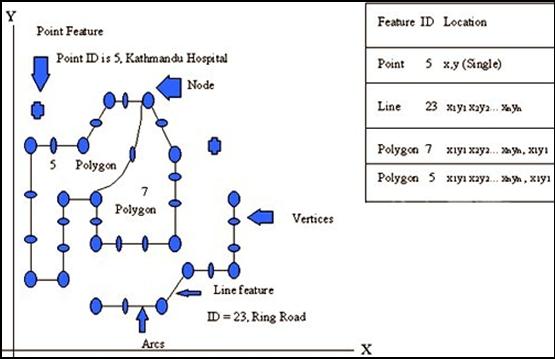
Figure 5.1: Spaghetti data model
Properties of Spaghetti Data Model
v Point is enclosed as single XY co-ordinate pair
v Line is encoded as a string of XY co-ordinate pairs
v Polygon is encoded as a closed loop of XY co-ordinates that define its boundary. The common boundary between adjacent polygons must be recorded twice, once for each polygon.
v The Spaghetti model is a file of spatial data constructed in this manner is essentially a collection of co-ordinate strings with no inherent structure-hence the term spaghetti model.
v Although all the spatial features are recorded the spatial relationships between these features are not encoded.
Topological model
The topological model is the most widely used method of encoding spatial relationships in a vector based GIS (Peuquet 1984). Topology is that branch of mathematics used to define spatial relationships between entities (ESRI 1992). For example, an area or polygon is defined by a set of lines which makes up its boundaries. In this case the line is the border between two polygons. Each line can represent part of a path connecting such other paths. For example, lines can be used to represent streets and the routes which pass along them. The connectivity or contiguity of these features is referred to as their topology structure (ESRI 1992). By sorting information about the location of a feature relative to other features, topology provides the basis for many kinds of geographic analysis without having access to the absolute locations held in the coordinate files (ESRI 1992).
Topology is the mathematical method used to define spatial relationships. The model is termed Arc-Node data model.
v Arc the basic logical entity, a series of point that starts and end at a node.
v Node is an intersection point where two or more arcs meet. A node can also occur at the end of a dangling arc i.e. and arc that is not connected to another arc such as the end of a dead-end street.
v Polygon is comprised of a closed chain of arcs that represents the boundary of the area.
v Point is encoded as a single XY co-ordinate pair. Point is considered as the polygon with no area.
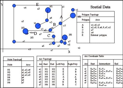
Figure 5.2: Topological Model
TIN data model
The Triangulated Irregular Network (TIN) data model is an alternative to the raster and vector data models for representing continuous surfaces. It allows surface models to be generated efficiently to analyze and display terrain and other types of surfaces. The TIN model creates a network of triangles by storing the topological relationships of the triangles. The fundamental building block of the TIN data is the node. Nodes are connected to their nearest neighbors by edges, according to a set of rules. Left-right topology is associated with the edges to identify adjacent triangles. The TIN creates triangles from a set of points called mass points, which always become nodes. The user is not responsible for selecting; all the nodes are added according to a set of rules. Mass points can be located anywhere, the more carefully selected, the more accurate the model of the surface will be. Well-placed mass points occur when there is a major change in the shape of the surface, for example, at the peak of a mountain, the floor of a valley, or at the edge (top and bottom) of cliffs. By connecting points on a valley floor or along the edge of a cliff, a linear break in the surface can be defined. These are called breaklines. Breaklines can control the shape of the surface model. They always form edges of triangles and, generally, cannot be moved. A triangle always has three and only three straight sides, making their representation rather simple. A triangle is assigned a unique identifier that defines by its three nodes and its two or three neighboring triangles (http://www.olemiss.edu/depts/geology/courses/ge
470/RasterDataModel.htm#The).
TIN is a vector-based topological data model that is used to represent terrain data. A TIN represents the terrain surface as a set of interconnected triangular facets. For each of the three vertices, the XY (geographic location) and the (elevation) Z values are encoded.
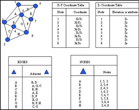
Figure 5.3: TIN Data Model
Four Tables for TIN Model
v Node Table it lists each triangle and the nodes which define it.
v Edge Table it lists three triangles adjacent to each facets. The triangles that border the boundary of the TIN show only two adjacent facets.
v XY Co-ordinate Table it lists the co-ordinate values of each node.
v Z Table it is the altitude value of each node.
Raster data models represent geographical space by dividing it in a series of units, each of which is limited and defined by an equal amount of earth's surface. These units are of different shapes, i.e. triangular or hexagonal, but the most commonly used shape is the square, called cell. Cells are interconnected to create plane surfaces representing all the space of a single area of study. The matrix of cells, organized into rows and columns is called a grid. In raster data model the focus is more in location. A raster data model is more like a photograph rather than a map. Geographic features are represented in grid cells or pixels filled with values. In the raster data model, the accuracy of the map depends on the scale of the map, the resolution and, hence, accuracy depends on the real world area represented by each grid cell.
(http://www.olemiss.edu/depts/geology/courses/ge470/RasterDataModel.htm#8b.1)
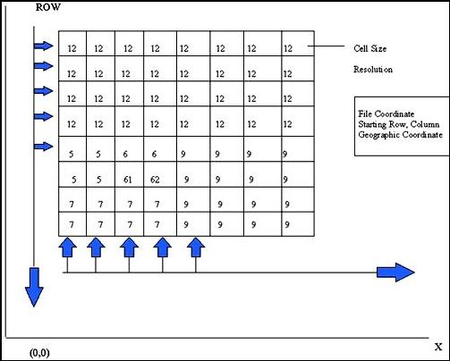
Figure 5.4: Raster Data Storage System
There are a number of ways of forcing a computer to store and reference the individual grid cell values, their attributes, coverage names and legends. The principal data structures existing in the market are:
1. Grid/Lunr/Magi
2. Imgrid GIS
3. Map Analysis Package (MAP)
In this model each grid cell is referenced or addressed individually and is associated with identically positioned grid cells in all other coverages, rather than like a vertical column of grid cells, each dealing with a separate theme. Comparisons between coverages are therefore performed on a single column at a time. Soil attributes in one coverage can be compared with vegetation attributes in a second coverage. Each soil grid cell in one coverage can be compared with a vegetation grid cell in the second coverage. The advantage of this data structure is that it facilitates the multiple coverage analysis for single cells. However, this limits the examination of spatial relationships between entire groups or themes in different coverages. (http://www.olemiss.edu/depts/geology/courses/ge470/RasterDataModel.htm#grid)
To represent a thematic map of land use that contains four categories: recreation, agriculture, industry and residence, each of these features have to be separated out as an individual layer. In the layer that represents agriculture 1 or 0 will represent the presence or absence of crops respectively. The rest of layer will be represented in the same way, with each variable referenced directly. The major advantage of IMGRID is its two-dimensional array of numbers resembling a map-like structure. The binary character of the information in each coverage simplifies long computations and eliminates the need for complex map legends. Since each coverage feature is uniquely identified, there is no limitation of assigning a single attribute value to a single grid cell. On the other side, the main problem related to information storage in an IMGRID structure is the excessive volume of data stored. Each grid cell will contain more than 1 or 0 values from more than one coverage and a large number of coverages are needed to store different types of information. (http://www.olemiss.edu/ depts/geology/courses/ge 470/RasterDataModel.htm#mgrid)
This type of data structure integrates the two structure discussed previously. In this raster structure, each thematic coverage is recorded and accessed separately by map name or title. This is accomplished by recording each variable, or mapping unit, of the coverage's theme as a separate number code or label, which can be accessed individually when the coverage is retrieved. The label corresponds to a portion of the legend has its own symbol assigned to it. This structure facilitates the performance of operations on individual grid cells and groups of similar cells, and the resulting changes in value require rewriting only a single number per mapping unit, simplifying the computations. The MAP data structure allows the manipulation of information in a many-to-one relationship of the attribute values and the sets of grids. The MAP is used in GIS mostly (http://www.olemiss.edu/depts/geology/courses/ge470/Raster DataModel.htm#Map).
Tessellation model
In the tessellation model the basic logical unit is a single cell or unit of space in a mesh (Star and Estes 1990). The location of geographic objects is defined by the row and column position of the cells that they occupy (Burrough 1986). The area that each cell represents defines the spatial resolution. The value assigned in the cell indicates the value of the attribute it represents. Hence, the essential property of such a data model is that spatial relations between logical units are implicit in the tessellation (Aronoff 1989).
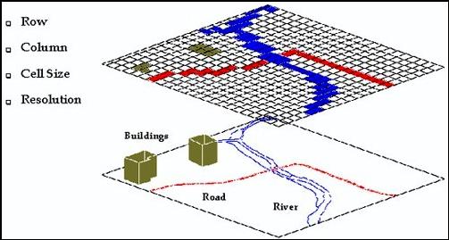
Figure 5.5: Conversion to Row and Cell
The integration of raster and vector data model is called hybrid data model.